Good day, folks!
Today I learned something about Excel — and yes, maybe some of you dah lama tahu… but sharing is caring, and learning never ends (especially when you’re a librarian, dad, gamer, and accidental spreadsheet warrior).

So here’s the situation:
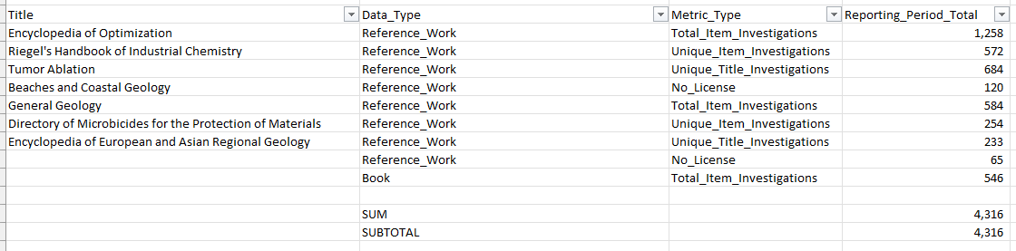
You use =SUM() to total up your data.
Then you apply a filter.
But… the total doesn’t change.
Why? Because SUM() includes everything — even rows you hid from your guilt.
Enter: Copilot. (See: This is how AI improves your puny human existence and makes you a more worthwhile version of yourself.)
Copilot said:
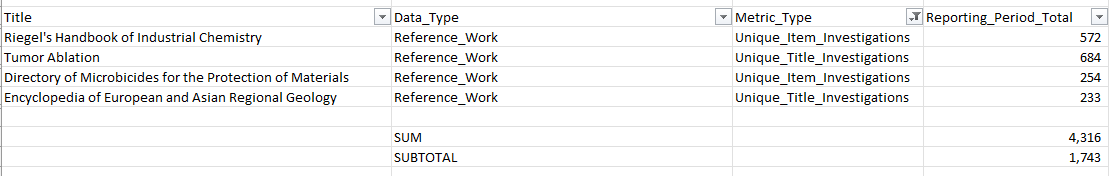
“Encik… if you want your totals to reflect only visible, filtered data — use
SUBTOTAL().”
Boom. Enlightenment. SUBTOTAL is basically SUM’s smarter sibling. It knows when to recalculate based on what you actually want to see — the visible rows.
Example:
Let’s say you’re tracking sales in column B (B2 to B100):
=SUBTOTAL(109, B2:B100)And yes… what is this mystical 109?
It’s a code — an operation indicator. In this case, 109 = SUM only visible rows.
It’s like function within a function — Excel’s version of Inception.
Here are more codes in the SUBTOTAL family:
- 101 → Average
- 102 → Count
- 104 → MAX
- 105 → MIN
So next time you’re slicing data like Amara punches psychos in Borderlands 3 — don’t just SUM(). SUBTOTAL() like a boss.
Milo in one hand. Filtered data in the other.
We move.